Confidence Interval

Definition

Confidence Interval
Let $X_{1}, X_{2}, \dots, X_{n}$ be a sample on a random variable $X$ , where $X$ has PDF $f (x; θ)$ , $θ \in Ω$ .
Let $L = L (X_{1}, \dots, X_{n})$ and $U = U (X_{1}, \dots, X_{n})$ be 2 statistics.
Given a level $α \in (0, 1)$ , if

P {L (X_{1}, \dots, X_{n}) \leq θ \leq U (X_{1}, \dots, X_{n})} = 1 - α

Then, $(L, U)$ is a $(1 - α) 100 %$ confidence interval for $θ$ .
The confidence coefficient of the interval is the probability that the interval includes $θ$ is $1 - α$ .

一个通俗版本的理解

If $P {{\hat{θ}}_{1} \leq θ \leq {\hat{θ}}_{2}} = 1 - α$ ,
Then, $[{\hat{θ}}_{1}, {\hat{θ}}_{2}]$ is the confidence interval of $θ$ with confidence coefficient $1 - α$ .

CI for Mean $μ$

Case 1: Normal Distribution （ $σ^{2}$ known）

$X_{i} \sim N (μ, σ^{2})$ and $σ^{2}$ is known.

\begin{aligned} \bar{X} & \sim N (μ, \frac{σ^{2}}{n}) \\ Z & = \frac{\bar{X} - μ}{\frac{σ}{\sqrt{n}}} \\ \sim N (0, 1) \\ P (- z_{\frac{α}{2}} \leq \frac{\bar{X} - μ}{\frac{σ}{\sqrt{n}}} \leq z_{\frac{α}{2}}) & = 1 - α \\ P {- z_{\frac{α}{2}} \leq \frac{\sqrt{n} (\bar{X} - μ)}{σ} \leq z_{\frac{α}{2}}} & = 1 - α \\ P {- σ z_{\frac{α}{2}} \leq \sqrt{n} (\bar{X} - μ) \leq σ z_{\frac{α}{2}}} & = 1 - α \\ P {- \frac{σ z_{\frac{α}{2}}}{\sqrt{n}} \leq \bar{X} - μ \leq \frac{σ z_{\frac{α}{2}}}{\sqrt{n}}} & = 1 - α \\ P {\bar{X} + \frac{σ z_{\frac{α}{2}}}{\sqrt{n}} \geq μ \geq \bar{X} - \frac{σ z_{\frac{α}{2}}}{\sqrt{n}}} & = 1 - α \\ P {μ \in [\bar{X} \pm \frac{σ z_{\frac{α}{2}}}{\sqrt{n}}]} & = 1 - α \end{aligned}

$(1 - α)$ CI: $[L (X_{1}, \dots, X_{n}), U (X_{1}, \dots, X_{n})]$ is random
Once the sample is observed,we can compute the sample mean $\bar{x}$

Note

TLDR: $\bar{x}$ 是随机变量 $\bar{X}$ 的一次观测值
$\bar{X}$ 是随机变量，所以 interval 是随机的；
一旦样本观测完，把 $\bar{X}$ 换成具体数字 $\bar{x}$ ，interval 就固定了

The computed interval, $\bar{x} \pm \frac{σ z_{\frac{α}{2}}}{\sqrt{n}}$ is $100 (1 - α) %$ , is confidence interval of $μ$

CI is centered at $\bar{x}$ (a point estimate of $μ$ )
Width: $2 z_{\frac{α}{2}} (\frac{σ}{\sqrt{n}})$

Note

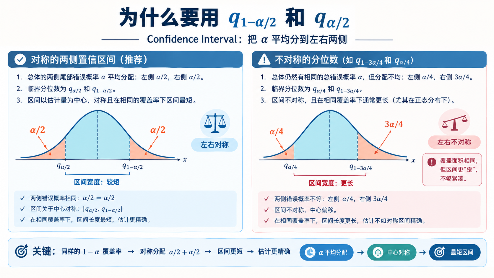
我们使用 $q_{1 - \frac{α}{2}}$ 和 $q_{\frac{α}{2}}$ 是为了让置信区间（Confidence Interval）左右对称。
这样不仅能最公平地分配误差，而且能让这个区间在数轴上变得最短，从而提高估计的精度。
$q_{1 - \frac{3}{4} α}, q_{\frac{α}{4}}$ 虽然覆盖的面积是对的，但会导致区间“歪”向一边，不够精准。

Fixed	Change	Width
$α, σ$	$n ↑$	$↓$
$σ, n$	$α ↓$	$↑$
$α, n$	$σ ↑$	$↑$

Example

Let $X$ be the length of lifetime of a light bulb and assume $X \sim N (μ, 1296)$ .
There are random sample of $n = 27$ with $\bar{x} = 1478$ .
What is the $95 %$ confidence interval?

\begin{aligned} 1 - α & = 0.95 \\ α & = 0.05 \\ \bar{X} & \sim N (μ, \frac{1296}{27}) \\ \sim N (μ, 48) \\ Z & = \frac{\bar{X} - μ}{\sqrt{48}} \sim N (0, 1) \\ P {- z_{\frac{0.05}{2}} \leq \frac{\bar{X} - μ}{\sqrt{48}} \leq z_{\frac{0.05}{2}}} & = 0.95 \\ P {z_{0.025} \sqrt{48} + \bar{X} \geq μ \geq \bar{X} - z_{0.025} \sqrt{48}} & = 0.95 \\ P {\bar{X} - z_{0.025} \sqrt{48} \leq μ \leq \bar{X} + z_{0.025} \sqrt{48}} & = 0.95 \\ P {\bar{X} - 1.96 \sqrt{48} \leq μ \leq \bar{X} + 1.96 \sqrt{48}} & = 0.95 \\ The confidence interval for μ & = [\bar{x} - 13.579, 13.579 + \bar{x}] \\ = [1478 - 13.579, 13.579 + 1478] \\ = [1464.42, 1491.58] \end{aligned}

Estimation Error

Estimation error $E := | \bar{x} - μ |$

Note

If it is normal distribution and $σ^{2}$ is known,
then

E \leq z_{\frac{α}{2}} \frac{σ}{\sqrt{n}}

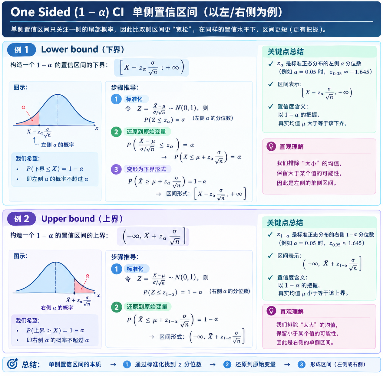
One Sided $(1 - α)$ CI

Example 1: Lower bound

\begin{aligned} P {θ \geq L (X_{1}, \dots, X_{n})} & = 1 - α \\ P {h (X_{1}, \dots, X_{n}; θ) \leq q_{α}} & = 1 - α \\ h (X_{1}, \dots, X_{n}; θ) & \sim N (0, 1) \\ P {\frac{\sqrt{n} (\bar{X} - μ)}{σ} \leq z_{α}} & = 1 - α \\ P {\bar{X} - μ \leq \frac{σ z_{α}}{\sqrt{n}}} & = 1 - α \\ P {μ \geq \bar{X} - z_{α} \frac{σ}{\sqrt{n}}} & = 1 - α \end{aligned}

The confidence interval is $[\bar{x} - z_{α} \frac{σ}{\sqrt{n}}, + \infty)$

Example 2: Upper bound

\begin{aligned} P {θ \leq U (X_{1}, \dots, X_{n})} & = 1 - α \\ P {h (X_{1}, \dots, X_{n}; θ) \geq q_{1 - α}} & = 1 - α \\ h (X_{1}, \dots, X_{n}; θ) & \sim N (0, 1) \\ P {\frac{\sqrt{n} (\bar{X} - μ)}{σ} \geq - z_{α}} & = 1 - α \\ P {\bar{X} - μ \geq - \frac{σ}{\sqrt{n}} z_{α}} & = 1 - α \\ P {\bar{X} + z_{α} \frac{σ}{\sqrt{n}} \geq μ} & = 1 - α \end{aligned}

Hence, confidence interval is $(- \infty, \bar{X} + z_{α} \frac{σ}{\sqrt{n}}]$

Case 2: Non-Normal Distribution ( $σ^{2}$ Known)

$X_{1}, \dots, X_{n}$ are i.i.d. with mean $μ = E (X_{1})$ and variance $σ^{2} = V a r (X_{1})$ , which is known.
By Central Limit Theorem, for large $n$ ,

\frac{\bar{X} - μ}{\frac{σ}{\sqrt{n}}} \overset{a p p r o x}{\sim} N (0, 1)

Thus,

P (\bar{X} - z_{\frac{α}{2}} \frac{σ}{\sqrt{n}} \leq μ \leq \bar{X} + z_{\frac{α}{2}} \frac{σ}{\sqrt{n}}) \approx 1 - α

The asymptotic / approximate two-sided $100 (1 - α) %$ CI is

\bar{x} \pm z_{\frac{α}{2}} (\frac{σ}{\sqrt{n}})

Example

Let $X$ be amount of orange juice consumed by an American per day
Given $σ = 96, n = 576, \bar{x} = 133$
What is the approximate 90% confidence interval for $μ$

\begin{aligned} 1 - α & = 0.9 \\ α & = 0.1 \\ By CLT, \frac{\bar{X} - μ}{\frac{96}{\sqrt{576}}} & \overset{a p p r o x}{\sim} N (0, 1) \\ \frac{\bar{X} - μ}{4} & \overset{a p p r o x}{\sim} N (0, 1) \\ P {- z_{\frac{α}{2}} \leq \frac{\bar{X} - μ}{4} \leq z_{\frac{α}{2}}} & = 0.9 \\ P {4 z_{0.05} + \bar{X} \geq μ \geq \bar{X} - 4 z_{0.05}} & = 0.9 \\ P {\bar{X} - 4 z_{0.05} \leq μ \leq \bar{X} + 4 z_{0.05}} & = 0.9 \\ The confidence interval for μ & = [\bar{x} \pm 4 z_{0.05}] \\ = [133 \pm 4 \times 1.645] \\ = [126.42, 139.58] \end{aligned}

Tip

Case 1 和 Case 2 做法几乎一样 ——
Substitute given variables and find the interval

\bar{x} \pm z_{\frac{α}{2}} (\frac{σ}{\sqrt{n}})

Case 3: Normal Distribution ( $σ^{2}$ Unknown)

$X_{1}, \dots, X_{n} \sim N (μ, σ^{2})$ and $σ^{2}$ is unknown
In #Case 1 Normal Distribution （$ sigma 2$ known）, $\bar{x} \pm z_{\frac{α}{2}} (\frac{σ}{\sqrt{n}})$ depends on $σ$ .
As $σ$ is unknown, we cannot use $\bar{x} \pm z_{\frac{α}{2}} (\frac{σ}{\sqrt{n}})$ to find the interval.
Hence, we need to use sample variance $S^{2}$ and Student's theorem

\begin{aligned} Sample variance: S^{2} & = \frac{1}{n - 1} \sum_{i = 1}^{n} (X_{i} - \bar{X})^{2} \\ Student’s theorem: \frac{\bar{X} - μ}{\frac{S}{\sqrt{n}}} & \sim t (n - 1) \end{aligned}

Hence, we need to use $\pm t_{\frac{α}{2}} (n - 1)$ as upper and lower bound.

\begin{aligned} P {- t_{\frac{α}{2}} (n - 1) \leq \frac{\bar{X} - μ}{\frac{S}{\sqrt{n}}} \leq t_{\frac{α}{2}} (n - 1)} & = 1 - α \\ P {- \frac{S \cdot t_{\frac{α}{2}} (n - 1)}{\sqrt{n}} \leq \bar{X} - μ \leq \frac{S \cdot t_{\frac{α}{2}} (n - 1)}{\sqrt{n}}} & = 1 - α \\ P {\bar{X} - \frac{S \cdot t_{\frac{α}{2}} (n - 1)}{\sqrt{n}} \leq μ \leq \bar{X} + \frac{S \cdot t_{\frac{α}{2}} (n - 1)}{\sqrt{n}}} & = 1 - α \end{aligned}

The $100 (1 - α) %$ CI of $μ$ is

[\bar{x} - \frac{s \cdot t_{\frac{α}{2}} (n - 1)}{\sqrt{n}}, \bar{x} + \frac{s \cdot t_{\frac{α}{2}} (n - 1)}{\sqrt{n}}]

Note

$S$ 和 $s$ 的区别跟 $X$ 和 $x$ 的区别一样 ——
即 $S$ 是 random variable，而 $s$ 是 observed value

Example

Let $X \sim N (μ, σ^{2})$ , and both $μ$ and $σ^{2}$ are unknown
Given $n = 20, \bar{x} = 507.5, s = 89.75, t_{0.05} (19) = 1.729$ .
What is 90% CI for $μ$ ?

\begin{aligned} 1 - α & = 0.9 \\ α & = 0.1 \\ \frac{\bar{X} - μ}{\frac{S}{\sqrt{20}}} \sim t (19) \\ P {- t_{\frac{0.1}{2}} (19) \leq \frac{\bar{X} - μ}{\frac{S}{\sqrt{20}}} \leq t_{\frac{0.1}{2}} (19)} & = 0.9 \\ P {- \frac{S \cdot t_{0.05} (19)}{\sqrt{20}} \leq \bar{X} - μ \leq \frac{S \cdot t_{0.05} (19)}{\sqrt{20}}} & = 0.9 \\ P {\bar{X} - \frac{S \cdot t_{0.05} (19)}{\sqrt{20}} \leq μ \leq \bar{X} + \frac{S \cdot t_{0.05} (19)}{\sqrt{20}}} & = 0.9 \\ The confidence interval for μ & = [\bar{x} \pm \frac{s \cdot t_{0.05} (19)}{\sqrt{20}}] \\ = [507.5 \pm \frac{89.75 \times 1.729}{\sqrt{20}}] \\ = [472.80, 542.20] \end{aligned}

Case 4: Non-Normal Distribution ( $σ^{2}$ Unknown)

$X_{1}, \dots, X_{n}$ are i.i.d. with mean $μ = E (X_{1})$ and variance $σ^{2} = V a r (X_{1})$ , which is unknown.
If $n$ is large enough / each $X_{i}$ is approximately normal, then

\frac{\bar{X} - μ}{\frac{S}{\sqrt{n}}} \overset{a p p r o x}{\sim} t (n - 1)

Approximate two-sided $100 (1 - α) %$ CI of $μ$ is

[\bar{x} - \frac{s \cdot t_{\frac{α}{2}} (n - 1)}{\sqrt{n}}, \bar{x} + \frac{s \cdot t_{\frac{α}{2}} (n - 1)}{\sqrt{n}}]

Important

If $n$ is large enough, then

t_{\frac{α}{2}} (n - 1) \approx z_{\frac{α}{2}}

Hence, the approximate two-sided $100 (1 - α) %$ CI for $μ$ is

[\bar{x} - z_{\frac{α}{2}} (\frac{s}{\sqrt{n}}), \bar{x} + z_{\frac{α}{2}} (\frac{s}{\sqrt{n}})]

Distribution of $X_{i}$	Distribution	Two-sided $1 - α$ CI
$N (μ, σ^{2})$ , $σ^{2}$ known	$\frac{\bar{X} - μ}{σ / \sqrt{n}} \sim N (0, 1)$	$\bar{x} \pm \frac{σ \cdot z_{α / 2}}{\sqrt{n}}$
Any distribution with large $n$ , $σ^{2}$ known	$\frac{\bar{X} - μ}{σ / \sqrt{n}} \overset{approx}{\sim} N (0, 1)$	$\bar{x} \pm \frac{σ \cdot z_{α / 2}}{\sqrt{n}}$
$N (μ, σ^{2})$ , $σ^{2}$ unknown	$\frac{\bar{X} - μ}{S / \sqrt{n}} \sim t (n - 1)$	$\bar{x} \pm \frac{s \cdot t_{α / 2} (n - 1)}{\sqrt{n}}$
Any distribution with large $n$ , $σ^{2}$ unknown	$\frac{\bar{X} - μ}{S / \sqrt{n}} \overset{approx}{\sim} t (n - 1)$	$\bar{x} \pm \frac{s \cdot t_{α / 2} (n - 1)}{\sqrt{n}}$

CI for the Difference of 2 Means

For

\begin{aligned} X_{1}, \dots, X_{n} & \sim N (μ_{X}, σ_{X}^{2}) \\ Y_{1}, \dots, Y_{m} & \sim N (μ_{Y}, σ_{Y}^{2}) \end{aligned}

To construct confidence intervals for $μ_{X} - μ_{Y}$ , we need to consider 3 cases

Pooled $t$ -interval
- $X_{1}, \dots, X_{n}, Y_{1}, \dots, Y_{m}$ are independent
- $σ_{X}^{2} = σ_{Y}^{2} = σ^{2}$
- $σ^{2}$ is unknown
Welch's $t$ -interval
- $X_{1}, \dots, X_{n}, Y_{1}, \dots, Y_{m}$ are independent
- $σ_{X}^{2} \neq σ_{Y}^{2}$ are both unknown
Paired $t$ -interval
- $X_{i}, Y_{i}$ are dependent for each $i$
- Pairs $(X_{i}, Y_{i})$ are independent
- $σ_{X}^{2}, σ_{Y}^{2}$ are unknown

Case 1: Pooled $t$ -interval

Let $X_{1}, \dots, X_{n} \sim N (μ_{X}, σ^{2})$ and $Y_{1}, \dots, Y_{m} \sim N (μ_{Y}, σ^{2})$ be independent random variables.
Then, $100 (1 - α) %$ CI for $μ_{X} - μ_{Y}$ is

\bar{X} - \bar{Y} \pm t_{\frac{α}{2}} (n + m - 2) S_{p} \sqrt{\frac{1}{n} + \frac{1}{m}}

$S_{p}^{2}$ is pooled estimator of $σ^{2}$ , which is unbiased estimator of $σ^{2}$

S_{p}^{2} = \frac{(n - 1) S_{X}^{2} + (m - 1) S_{Y}^{2}}{n + m - 2} = \frac{\sum_{i = 1}^{n} (X_{i} - \bar{X})^{2} + \sum_{i = 1}^{m} (Y_{i} - \bar{Y})^{2}}{n + m - 2}

Example

Let $X \sim N (μ x, σ^{2})$ be the score on a standardized test in a large high school.
Let $Y \sim N (μ_{Y}, σ^{2})$ be the score on a standardized test in a small high school.
Given:
$n = 9, \bar{x} = 81.31, s_{x}^{2} = 60.76$
$m = 15, \bar{y} = 78.61, s_{y}^{2} = 48.24$
What is 95% confidence interval for $μ_{x} - μ_{y}$

\begin{aligned} 1 - α & = 0.95 \\ α & = 0.05 \\ n + m - 2 & = 22 \\ t_{\frac{1 - 0.95}{2}} (22) & = 2.074 \\ t_{0.025} (22) & = 2.074 \\ s_{p}^{2} & = \frac{8 (60.76) + 14 (48.24)}{22} \\ s_{p} & = \sqrt{\frac{486.08 + 675.36}{22}} \\ Confidence interval for μ_{X} - μ_{Y} & = 81.31 - 78.61 \pm 2.074 (\sqrt{\frac{486.08 + 675.36}{22}}) (\sqrt{\frac{1}{9} + \frac{1}{15}}) \\ = [- 3.65, 9.05] \end{aligned}

Case 2: Welch's $t$ -interval

Let $X_{1}, \dots, X_{n} \sim N (μ_{X}, σ_{X}^{2}), Y_{1}, \dots, Y_{m} \sim N (μ_{Y}, σ_{Y}^{2})$ be independent
Approximate $100 (1 - α) %$ CI for $μ_{X} - μ_{Y}$ is

\bar{X} - \bar{Y} \pm t_{\frac{α}{2}} (r) \sqrt{\frac{S_{X}^{2}}{n} + \frac{S_{Y}^{2}}{m}}

where

r = ⌊ \frac{{(\frac{S_{X}^{2}}{n} + \frac{S_{Y}^{2}}{m})}^{2}}{\frac{1}{n - 1} {(\frac{S_{X}^{2}}{n})}^{2} + \frac{1}{m - 1} {(\frac{S_{Y}^{2}}{m})}^{2}} ⌋

Note

$⌊ x ⌋$ is floor function (round down)
i.e. $⌊ 3.4 ⌋ = ⌊ 3.9 ⌋ = 3$

Note

Welch 公式算出来的自由度 $r$ 通常不是整数（比如 19.8），但 t 分布表只有整数自由度，必须取一个整数去查表
而「向下取整」比「向上取整/四舍五入」更保守、更安全--它让区间更宽，绝不会把真实置信水平说低

Example

Assume $σ_{X}^{2} \neq σ_{Y}^{2}$
Scenario is same as #^fd6a48

\begin{aligned} α & = 0.05 \\ r & = ⌊ \frac{{(\frac{60.76}{9} + \frac{48.24}{15})}^{2}}{\frac{1}{8} {(\frac{60.76}{9})}^{2} + \frac{1}{14} {(\frac{48.24}{15})}^{2}} ⌋ \\ = 15 \\ t_{0.025} (15) & = 2.131 \\ Welch’s t -interval for μ_{X} - μ_{Y} & = 81.31 - 78.61 \pm 2.131 (\sqrt{\frac{60.76}{9} + \frac{48.24}{15}}) \\ = [- 4.0278, 9.4278] \end{aligned}

Compared to pooled $t$ -interval $[- 3.65, 9.05]$ , Welch's $t$ -interval is wider than pooled $t$ -interval.

Case 3: Paired $t$ -interval

Definition

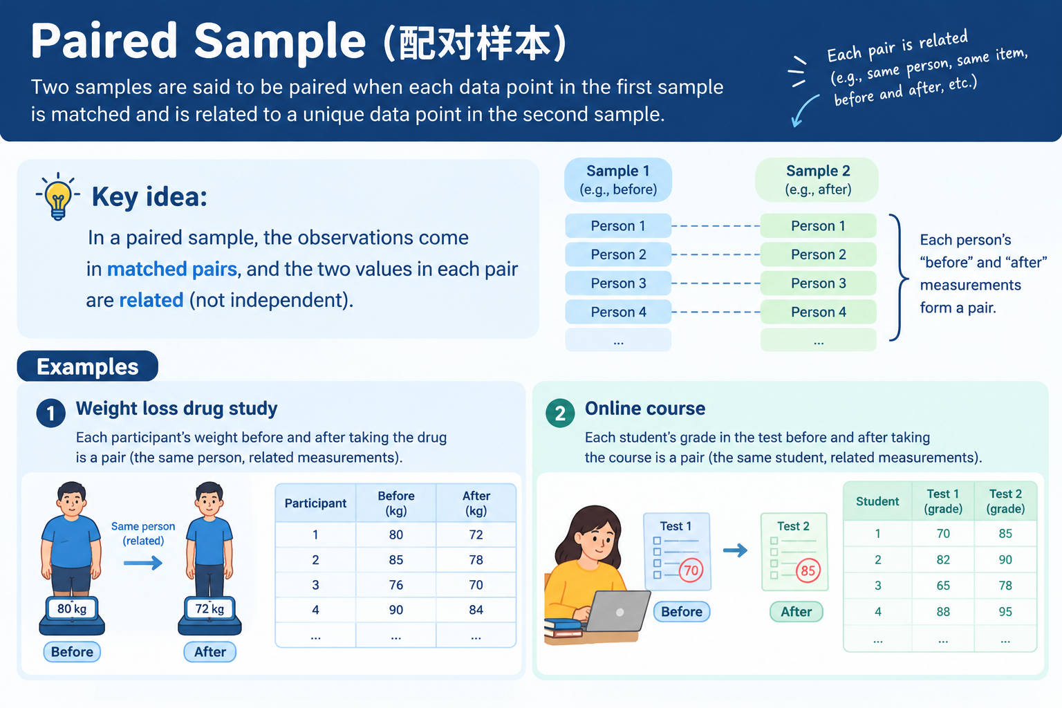
Paired samples
Each data point in the first sample is matched & related to a unique data point in the second sample

Let $(X_{1}, Y_{1}), \dots, (X_{n}, Y_{n})$ be $n$ pairs of dependent measures.
Let $D_{i} = X_{i} - Y_{i}$ .
Suppose $D_{1}, \dots, D_{n} \sim N (μ_{D}, σ_{D}^{2})$ with $μ_{D} = μ_{X} - μ_{Y}$ .
Then, $100 (1 - α) %$ CI for $μ_{X} - μ_{Y}$ is

\bar{D} \pm t_{\frac{α}{2}} (n - 1) \frac{S_{D}}{\sqrt{n}}

where

\begin{aligned} \bar{D} & = \frac{1}{n} \sum_{i = 1}^{n} D_{i} \\ S_{D}^{2} & = \frac{1}{n - 1} \sum_{i = 1}^{n} (D_{i} - \bar{D})^{2} \end{aligned}

Note

配对的目的是“消掉个体之间的差异”
以减肥药为例 —— 有人天生体重就高（比如 90 kg），有人天生低（比如 50 kg）。
如果我用"服药后组 vs 服药前组"来比，即使药完全无效，两组的个体构成稍有不同（比如高体重的人恰好多分了几个到"服药后"组），均值就会差出好几公斤。
这个"个体差异"造成的噪声，把真正的药效完全盖住了。

配对的做法是同一个人自己和自己比： $D_{i} = {服药后}_{i} - {服药前}_{i}$ 。
这个差值里，"这个人天生体重多少"被减掉了 —— 它同时出现在 $X_{i}$ 和 $Y_{i}$ 里，一减就没了。
剩下的 $D_{i}$ 只包含"药效 + 这一次测量的随机误差"。

Example

An experiment was conducted to compare people's reaction times to a red light versus green light.
When signaled with either red or green light, the subject was asked to hit a switch to turn off the light
When the switch was hit, a clock was turned off and the reaction time was recorded

Given $n = 8, \bar{d} = - 0.062, s_{d} = 0.0765$
What is the 95% CI for $μ_{X} - μ_{Y}$ ?

Subject	Red ( $x$ )	Green ( $y$ )	$d = x - y$
1	0.30	0.43	−0.13
2	0.23	0.32	−0.09
3	0.41	0.58	−0.17
4	0.53	0.46	0.07
5	0.24	0.27	−0.03
6	0.36	0.41	−0.05
7	0.38	0.38	0.00
8	0.51	0.61	−0.10

\begin{array}{r} - 0.0625 \pm t_{0.025} (7) (\frac{0.0765}{\sqrt{8}}) = [- 0.1265, 0.0015] \end{array}

Using pooled and Welch's $t$ -interval to calculate CI,
Given that $\bar{x} = 0.3700, \bar{y} = 0.4325, s_{X} = 0.1124, s_{Y} = 0.1173$ .
Pooled $t$ -interval

\begin{aligned} 95 % C I & = 0.3700 - 0.4325 \pm t_{0.025} (14) \sqrt{\frac{7 (0.1124)^{2} + 7 (0.1173)^{2}}{14}} \sqrt{\frac{2}{8}} \\ = [- 0.1857, 0.0607] \end{aligned}

Welch's $t$ -interval

\begin{aligned} r & = ⌊ \frac{{(\frac{{0.1124}^{2}}{8} + \frac{{0.1173}^{2}}{8})}^{2}}{\frac{1}{7} {(\frac{{0.1124}^{2}}{8})}^{2} + \frac{1}{7} {(\frac{{0.1173}^{2}}{8})}^{2}} ⌋ \\ = 13 \\ 95 % C I & = 0.3700 - 0.4325 \pm t_{0.025} (13) \sqrt{\frac{{0.1124}^{2}}{8} + \frac{{0.1173}^{2}}{8}} \\ = [- 0.1865, 0.0615] \end{aligned}

With same center $\bar{d} = \bar{x} - \bar{y}$ , CI widths are different
In general, CI width: Pair $t$ -interval < Pool $t$ -interval < Welch's $t$ -interval

Note

When $s_{X}^{2}$ is closed to $s_{Y}^{2}$ , widths of pooled $t$ -interval and Welch's $t$ -interval are similar.

CI for Proportions

Example

In a political campaign survey, we collect a sample of $n = 351$ voters.
$y = 185$ out of them favor candidate A and remaining favour candidate B.
Let $p$ be the supporting rate in the population.
How to build a CI for the supporting rate?

\begin{aligned} Let X_{i} & = {\begin{cases} 1, & favour candidate A \\ 0, & favour candidate B \end{cases} \\ X_{1}, \dots, X_{n} & \sim Bernoulli (p) \\ Denote Y & = \sum_{i = 1}^{n} X_{i} \sim Bin (n, p) \\ By CLT, \frac{Y - n p}{\sqrt{n p (1 - p)}} & \overset{approx}{\sim} N (0, 1) \\ By MLE, \\ L (p) & = \prod_{i = 1}^{n} p^{X_{i}} (1 - p)^{1 - X_{i}} \\ = p^{\sum_{i = 1}^{n} X_{i}} (1 - p)^{n - \sum_{i = 1}^{n} X_{i}} \\ = p^{Y} (1 - p)^{n - Y} \\ ℓ (p) & = Y \ln p + (n - Y) \ln (1 - p) \\ ℓ^{'} (p) & = 0 \\ \frac{Y}{p} - \frac{n - Y}{1 - p} & = 0 \\ \frac{Y}{p} & = \frac{Y - n}{p - 1} \\ Y (p - 1) & = p (Y - n) \\ Y p - Y & = p Y - p n \\ \hat{p} & = \frac{Y}{n} \\ = \frac{185}{351} \\ \approx 0.527 \\ Y & = n \hat{p} \\ P {- z_{\frac{α}{2}} \leq \frac{Y - n p}{\sqrt{n p (1 - p)}} \leq z_{\frac{α}{2}}} & \approx 1 - α \\ P {- z_{\frac{α}{2}} \leq \frac{n (\hat{p} - p)}{\sqrt{n} \sqrt{p (1 - p)}} \leq z_{\frac{α}{2}}} & \approx 1 - α \\ P {- z_{\frac{α}{2}} \leq \frac{\sqrt{n} (\hat{p} - p)}{\sqrt{p (1 - p)}} \leq z_{\frac{α}{2}}} & \approx 1 - α \\ P {- z_{\frac{α}{2}} \leq \frac{\hat{p} - p}{\sqrt{\frac{p (1 - p)}{n}}} \leq z_{\frac{α}{2}}} & \approx 1 - α \\ P {- z_{\frac{α}{2}} \sqrt{\frac{p (1 - p)}{n}} \leq \hat{p} - p \leq z_{\frac{α}{2}} \sqrt{\frac{p (1 - p)}{n}}} & \approx 1 - α \\ P {\hat{p} - z_{\frac{α}{2}} \sqrt{\frac{p (1 - p)}{n}} \leq p \leq \hat{p} + z_{\frac{α}{2}} \sqrt{\frac{p (1 - p)}{n}}} & \approx 1 - α \end{aligned}

By Law of Large Number, $\hat{p} \to p$ .
Hence, we can use $\hat{p}$ to approximate $p$ when $n$ is large.
Then, the approximate $100 (1 - α) %$ CI is

\hat{p} \pm z_{\frac{α}{2}} \sqrt{\frac{\hat{p} (1 - \hat{p})}{n}}

Therefore,

\begin{aligned} \hat{p} & \approx 0.527 \\ z_{0.025} & = 1.96 \\ Approximate 95 % CI for p & = 0.527 \pm 1.96 \sqrt{\frac{0.527 (1 - 0.527)}{351}} \\ = [0.475, 0.579] \end{aligned}

To measure the difference in proportions between 2 independent populations,

$p_{i}$ : Proportion in population $i$ with a characteristic ( $\frac{Y_{i}}{n_{i}}$ )
$Y_{i}$ : No. of successes in sample from population $i$
$n_{i}$ : Sample size in population $i$

\begin{aligned} E (\frac{Y_{i}}{n_{i}}) & = p_{i} \\ V a r (\frac{Y_{i}}{n_{i}}) & = \frac{p_{i} (1 - p_{i})}{n_{i}} \end{aligned}

Hence,

\begin{aligned} E (\frac{Y_{1}}{n_{1}} - \frac{Y_{2}}{n_{2}}) & = p_{1} - p_{2} \\ V a r (\frac{Y_{1}}{n_{1}} - \frac{Y_{2}}{n_{2}}) & = \frac{p_{1} (1 - p_{1})}{n_{1}} + \frac{p_{2} (1 - p_{2})}{n_{2}} \end{aligned}

When $n_{1}$ and $n_{2}$ is large, by CLT,

\begin{aligned} {\hat{p}}_{1} - {\hat{p}}_{2} & \sim N (p_{1} - p_{2}, \frac{p_{1} (1 - p_{1})}{n_{1}} + \frac{p_{2} (1 - p_{2})}{n_{2}}) \\ \frac{({\hat{p}}_{1} - {\hat{p}}_{2}) - (p_{1} - p_{2})}{\sqrt{\frac{p_{1} (1 - p_{1})}{n_{1}} + \frac{p_{2} (1 - p_{2})}{n_{2}}}} & \sim N (0, 1) \\ P {- z_{\frac{α}{2}} \leq \frac{({\hat{p}}_{1} - {\hat{p}}_{2}) - (p_{1} - p_{2})}{\sqrt{\frac{p_{1} (1 - p_{1})}{n_{1}} + \frac{p_{2} (1 - p_{2})}{n_{2}}}} \leq z_{\frac{α}{2}}} & \approx 1 - α \end{aligned}

By Law of Large Number, we can approximate $p_{i}$ by $\hat{p}$ .
Hence, the approximate $100 (1 - α) %$ CI for $p_{1} - p_{2}$ is

{\hat{p}}_{1} - {\hat{p}}_{2} \pm z_{\frac{α}{2}} \sqrt{\frac{{\hat{p}}_{1} (1 - {\hat{p}}_{1})}{n_{1}} + \frac{{\hat{p}}_{2} (1 - {\hat{p}}_{2})}{n_{2}}}

Example

Let $p_{1}$ be the proportion of male students into gaming, and $p_{2}$ be the proportion of female students into gaming.
Suppose ${\hat{p}}_{1} = 0.6, {\hat{p}}_{2} = 0.4$ .
When $n_{1} = 2000, n_{2} = 2200$ , please construct approximate 95% CI for $p_{1} - p_{2}$ .

The approximated 95% CI for $p_{1} - p_{2}$ is given by

\begin{aligned} 0.6 - 0.4 \pm z_{0.025} \sqrt{\frac{0.6 (1 - 0.6)}{2000} + \frac{0.4 (1 - 0.4)}{2200}} & = 0.2 \pm 1.96 \sqrt{\frac{0.6 (0.4)}{2000} + \frac{0.4 (0.6)}{2200}} \\ = [0.17, 0.23] \end{aligned}

Sample Size Determination

动机： 由于样本量多会增加成本，而样本量少会影响预测的准确度。因此我们需要找出在指定精度下，最少的样本量是多少。

Normal Distribution ( $σ^{2}$ Known)

For $X_{1}, \dots, X_{n} \sim N (μ, σ^{2})$ and $σ^{2}$ is known, the $100 (1 - α) %$ CI for $μ$ is

\bar{x} \pm z_{\frac{α}{2}} \frac{σ}{\sqrt{n}}

$z_{\frac{α}{2}} \frac{σ}{\sqrt{n}}$ is called half-width, as well as margin of error or max. error of the estimate

Note

The smaller the half-width $z_{\frac{α}{2}} \frac{σ}{\sqrt{n}}$ , the more accurate the estimate.

We requires the half-width must be less than a given tolerance $ϵ$ in precision

\begin{aligned} z_{\frac{α}{2}} \frac{σ}{\sqrt{n}} & \leq ϵ \\ n & \geq \frac{z_{\frac{α}{2}}^{2} σ^{2}}{ϵ^{2}} \end{aligned}

Example

A psychology study uses standardized memory tests with known standard deviation $σ = 12$ .
Find the minimum sample size $n$ needed for a 95% confidence interval with a margin of error at most 2.

\begin{aligned} n & \geq \frac{z_{0.025}^{2} (12)^{2}}{2^{2}} \\ n & \geq 138.3 \end{aligned}

Hence, the minimum sample size is 139 students.

Normal Distribution ( $σ^{2}$ Unknown)

When $σ^{2}$ is unknown, the $100 (1 - α) %$ CI is

\bar{x} \pm t_{\frac{α}{2}} (n - 1) \frac{s}{\sqrt{n}}

$t_{\frac{α}{2}} (n - 1) \frac{s}{\sqrt{n}}$ is the half-width.
Hence,

\begin{aligned} t_{\frac{α}{2}} (n - 1) \frac{s}{\sqrt{n}} & \leq ϵ \\ n & \geq \frac{t_{\frac{α}{2}}^{2} (n - 1) s^{2}}{ϵ^{2}} \end{aligned}

However, there are 2 issues

$t_{\frac{α}{2}}^{2} (n - 1)$ depends on $n$ . Hence, we use $z_{\frac{α}{2}}$ to approximate $t_{\frac{α}{2}}^{2} (n - 1)$
$s^{2}$ depends on $n$ . Hence, we have to estimate $s_{p}^{2}$ from prior knowledge / pilot study
Finally,

n \geq \frac{z_{\frac{α}{2}}^{2} (s_{p}^{2})}{ϵ^{2}}

Proportion

The approximate CI for proportion $p$ is

\hat{p} \pm z_{\frac{α}{2}} \sqrt{\frac{\hat{p} (1 - \hat{p})}{n}}

Let the required precision be $ϵ$ .

\begin{aligned} z_{\frac{α}{2}} \sqrt{\frac{\hat{p} (1 - \hat{p})}{n}} & \leq ϵ \\ n & \geq \frac{z_{\frac{α}{2}}^{2} \hat{p} (1 - \hat{p})}{ϵ^{2}} \end{aligned}

However, $\hat{p}$ depends on $n$
Since $\hat{p}$ is unknown, we have 2 approach to approximate $\hat{p}$

Use prior estimate $p^{*}$ :
- 来自历史数据、以前的调查或者预试研究（pilot study）

n \geq \frac{z_{\frac{α}{2}}^{2} p^{*} (1 - p^{*})}{ϵ^{2}}

Use the max. variance
- As $p \in [0, 1]$ , $p (1 - p) \leq \frac{1}{4}$
- $p (1 - p)$ attains its maximum when $p = \frac{1}{2}$
- Hence, assume $\hat{p} = \frac{1}{2}$

\begin{aligned} n & \geq \frac{z_{\frac{α}{2}}^{2} \frac{1}{2} (1 - \frac{1}{2})}{ϵ^{2}} \\ \geq \frac{z_{\frac{α}{2}}^{2}}{4 ϵ^{2}} \end{aligned}

Proof

Prove $p (1 - p) \leq \frac{1}{4}$ by completing square.

\begin{aligned} p (1 - p) & = p - p^{2}, p \in [0, 1] \\ = - (p^{2} - p + \frac{1}{4}) + \frac{1}{4} \\ = - {(p - \frac{1}{2})}^{2} + \frac{1}{4} \\ ∴ p (1 - p) attains its maximum at & (\frac{1}{2}, \frac{1}{4}) \end{aligned}

Example

A particular area contains 8000 apartment units.
In a preliminary survey, 12% of the respondents said they planned to sell their apartments within the next year.
We want to estimate the interval for the total number of owners planning to sell.
Suppose that a 95% confidence interval with the half-width less than 200 is desired. How many owners do we need to survey.

From now, we have

$p^{*}$ : 12% (it is prior estimate)
$ϵ$ : 200
$α$ : 5%
As there are 8000 apartments in total, the approximate CI of the number of owners planning to sell has to multiply by 8000.

\begin{aligned} 8000 (z_{0.025} \sqrt{\frac{\hat{p} (1 - \hat{p})}{n}}) & \leq 200 \end{aligned}

Approximate $\hat{p}$ by $p^{*}$

\begin{aligned} 8000 (1.96 \sqrt{\frac{0.12 (1 - 0.12)}{n}}) & \leq 200 \\ 1.96 \sqrt{\frac{0.1056}{n}} & \leq 0.025 \\ n & \geq 649.077 \end{aligned}

Hence, we need to survey at least 650 apartment owners

CI for Mean μ

Case 1: Normal Distribution （σ2 known）

Example

Estimation Error

One Sided (1−α) CI

Example 1: Lower bound

Example 2: Upper bound

Case 2: Non-Normal Distribution (σ2 Known)

Example

Case 3: Normal Distribution (σ2 Unknown)

Example

Case 4: Non-Normal Distribution (σ2 Unknown)

CI for the Difference of 2 Means

Case 1: Pooled t-interval

Example

Case 2: Welch's t-interval

Example

Case 3: Paired t-interval

Example

CI for Proportions

Example

Example

Sample Size Determination

Normal Distribution (σ2 Known)

Example

Normal Distribution (σ2 Unknown)

Proportion

Example

CI for Mean $μ$

Case 1: Normal Distribution （ $σ^{2}$ known）

One Sided $(1 - α)$ CI

Case 2: Non-Normal Distribution ( $σ^{2}$ Known)

Case 3: Normal Distribution ( $σ^{2}$ Unknown)

Case 4: Non-Normal Distribution ( $σ^{2}$ Unknown)

Case 1: Pooled $t$ -interval

Case 2: Welch's $t$ -interval

Case 3: Paired $t$ -interval

Normal Distribution ( $σ^{2}$ Known)

Normal Distribution ( $σ^{2}$ Unknown)