Null hypothesis : Initial claim / assumption on the values that can take
通俗来说:没变化 / 维持现状
Alternative hypothesis : The competing claim / assumption against which we would like to test the initial claim / assumption
通俗来说:想证明的新发现
Tip
判决要么是"**reject 拒绝 **",要么是"fail to reject 未能拒绝 ",而不是"接受 "。
Simple hypothesis: Hypothesis in which only takes on 1 value
Composite hypothesis: Hypothesis in which takes on a range of value
Example
Let equal the breaking strength of a steel bar. If the bar is manufactured by process I, . It is hoped that if process II (a new process) is used, . Given a large number of steel bars manufactured by process II, how could we test whether the five-unit increase in the mean breaking strength was realized?
Judgement: 5-unit increase in or not
Simple null hypothesis :
Simple alternative hypothesis :
Composite null hypothesis :
Composite alternative hypothesis :
Types
直觉解释
Simple vs Simple
只关心两个精准数值
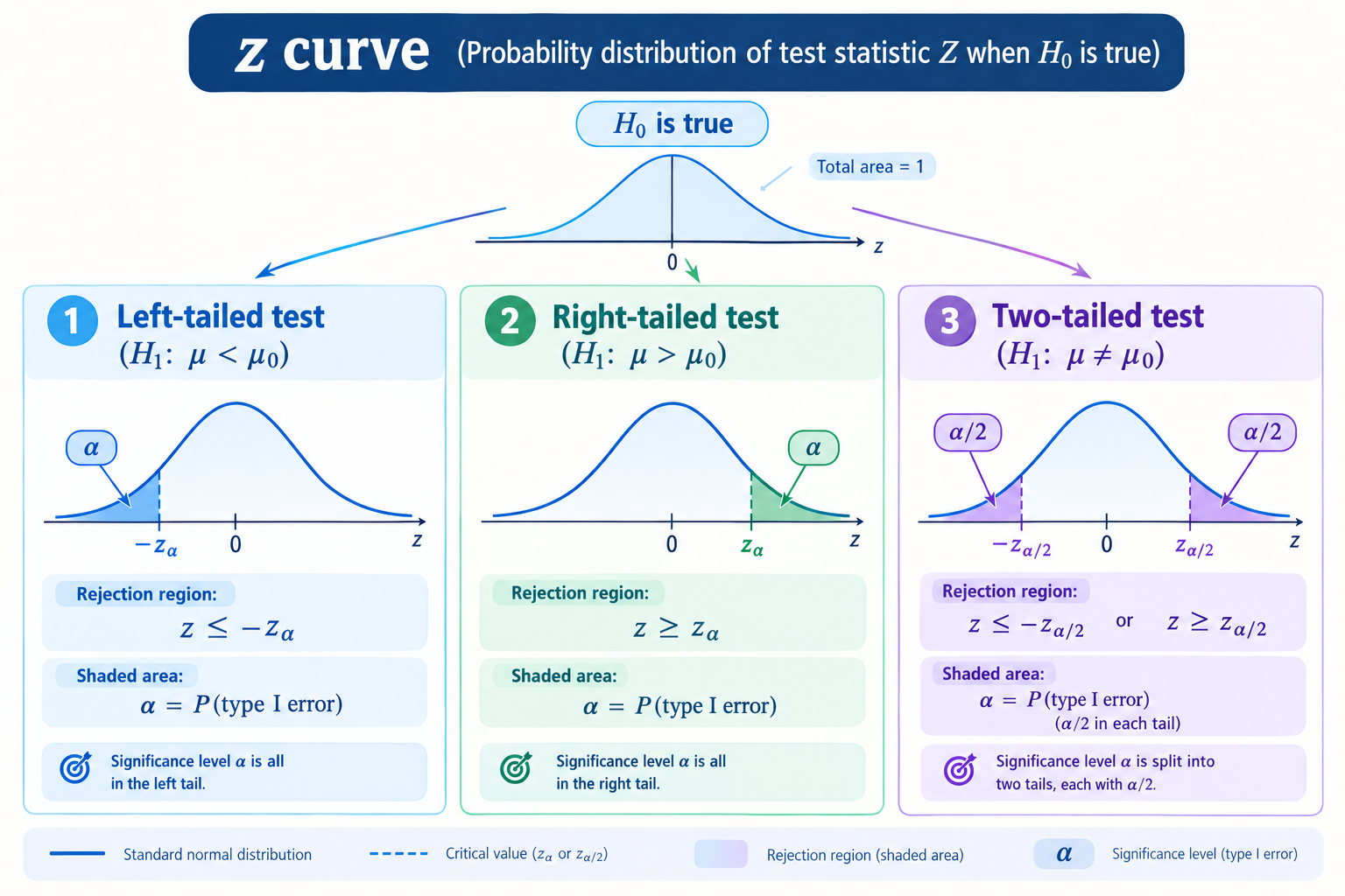
单侧 One-sided(右尾)
只关心"有没有变大"
单侧 One-sided(左尾)
只关心"有没有变小"
双侧 Two-sided(双尾)
变大变小都算异常
Composite vs Composite
覆盖全部数值
Critical Region and Test Statistic
The space of the sample
Tip
: 这次抽样所有可能出现的结果的 set
Hypothesis testing is based on critical region , which is subset of .
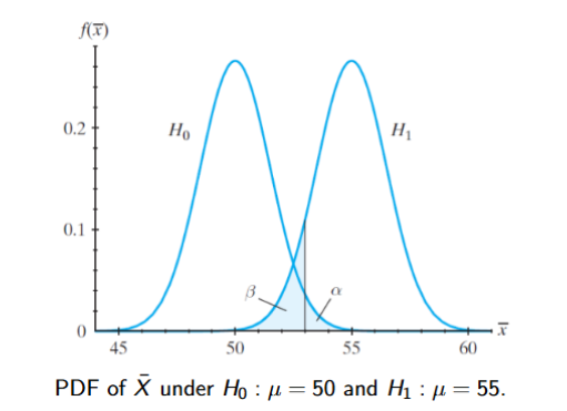
, Take critical region . What is the probability of type I error and type II error in the following test
Tip
哪怕真实均值就是 50,单凭抽样波动,也有约 2.28% 的概率 在 53 以上,被我们冤枉。
Tip
即便真实均值是 55,仍有约 9.12% 的概率没跨过 53 而漏报
Note
By changing critical region , and change in different direction (i.e. ). Hence, and cannot be reduced at the same time
Significance Level
We usually fix the probability of type I error , and then determine the corresponding critical region. In this scenario, the value of is called significance level of the test.
Tip
在先确定 type I error 的值,再决定 critical region 的情景下, 便称为 significance level
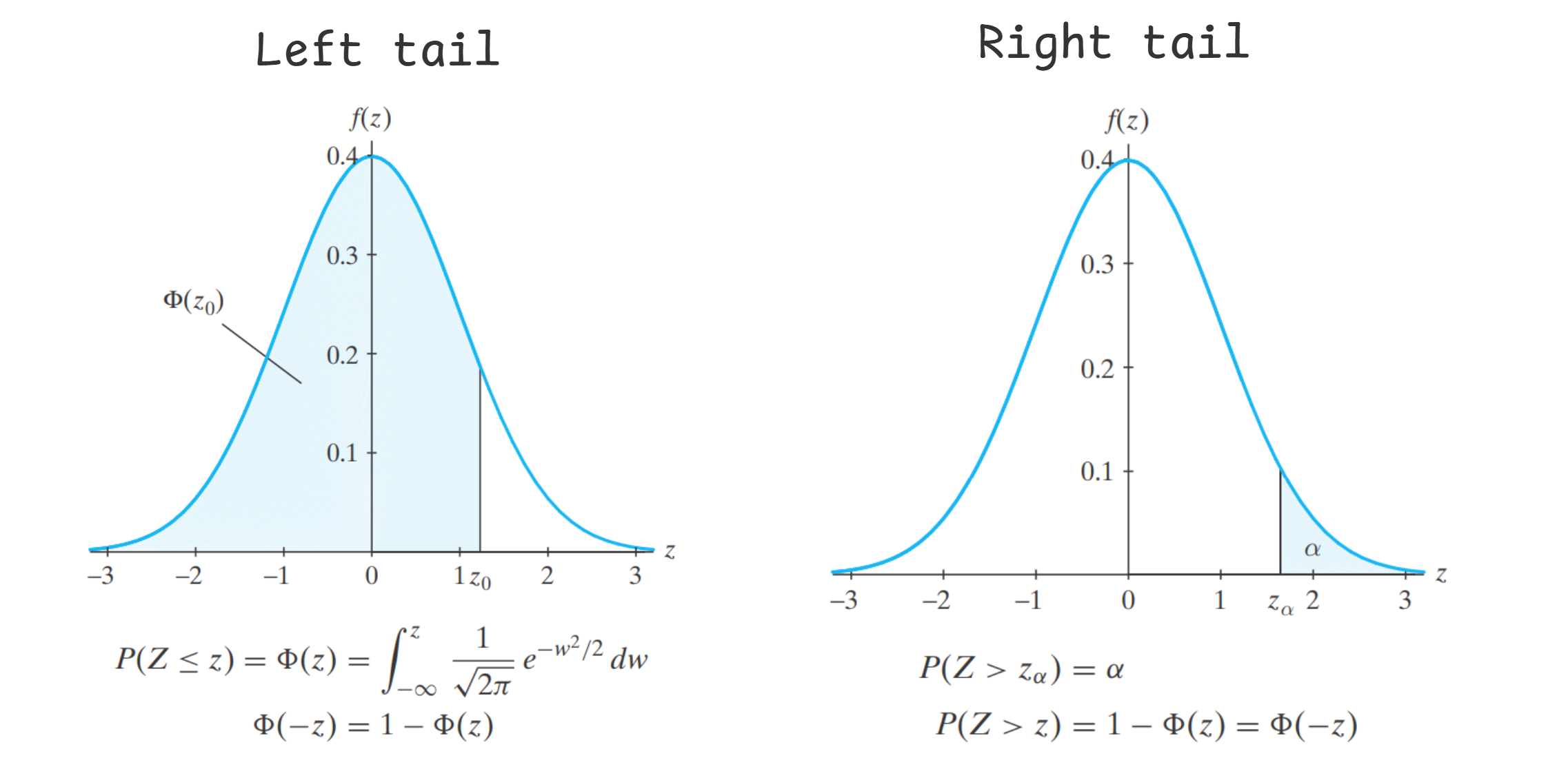
-value: If is true, the probability of observing a more extreme test statistic (favour ) Smaller -value indicates the data is more unlikely coming from and is perhaps better retained
Tip
想象一个场景:你抛一枚硬币 100 次,得到 90 次正面。你会怀疑硬币是不是被做手脚了(: 硬币公平 vs : 硬币不公平)。
Following the same example above (,). Given observed test statistics .
For versus
更极端方向是
For versus
更极端方向是
For versus
更极端方向是
For versus
更极端方向是 and
Hypothesis Testing for Normal Mean
There are 3 approaches to hypothesis testing
-value approach
Reject if -value
Critical region approach
Reject if statistic falls in critical region
Confidence interval approach
Reject if null value (value of null hypothesis) is not include in CI
Case 1: Known
Consider test statistic
Under ,
Tip
只是一个已知的、假设的数值。
当 被定义为 ,由于 并未假设为 ,因此 。
直到题目给出 "Under ",假定 为 时, 才服从 。
Once the data is observed, we can compute
Tip
is observed value of
Important
大写 = 随机变量(random variable)
小写 = 观测值(observed value / realization)
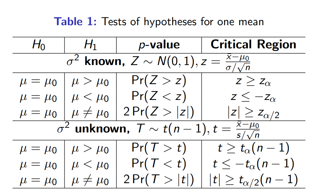
For the one-sided test
-value is
Reject at significance level when either
-value approach: OR
Critical region approach: OR
Confidence interval approach:
Tip
这三种 approach 都是等价的
For one-sided test
Reject at significance level when either
OR
OR
For two-sided test
Reject at significance level when either
OR
OR
Case 2: Unknown
When is unknown, replace standard normal distribution by -distribution with degree of freedom and by in #Case 1 $ sigma 2$ Known
Consider test statistic
Under , Once data are observed, we can compute
For the one-sided test
Reject at significance level when either
OR
OR
For the one-sided test
Reject at significance level when either
OR
For the two-sided test
Reject at significance level when either
Example
Two-sided Test
Let (in millimeters) equal the growth in 15 days of a tumor induced in a mouse. Assume that the distribution of is Test the null hypothesis against the two-sided alternative hypothesis Observe that observations with and set significance level of
Hence, we fail to reject at 10% significance level
One-sided Test
Suppose that we have Test against , given significance level
Test Equality of Two Normal Means
Settings
2 populations with i.i.d. samples
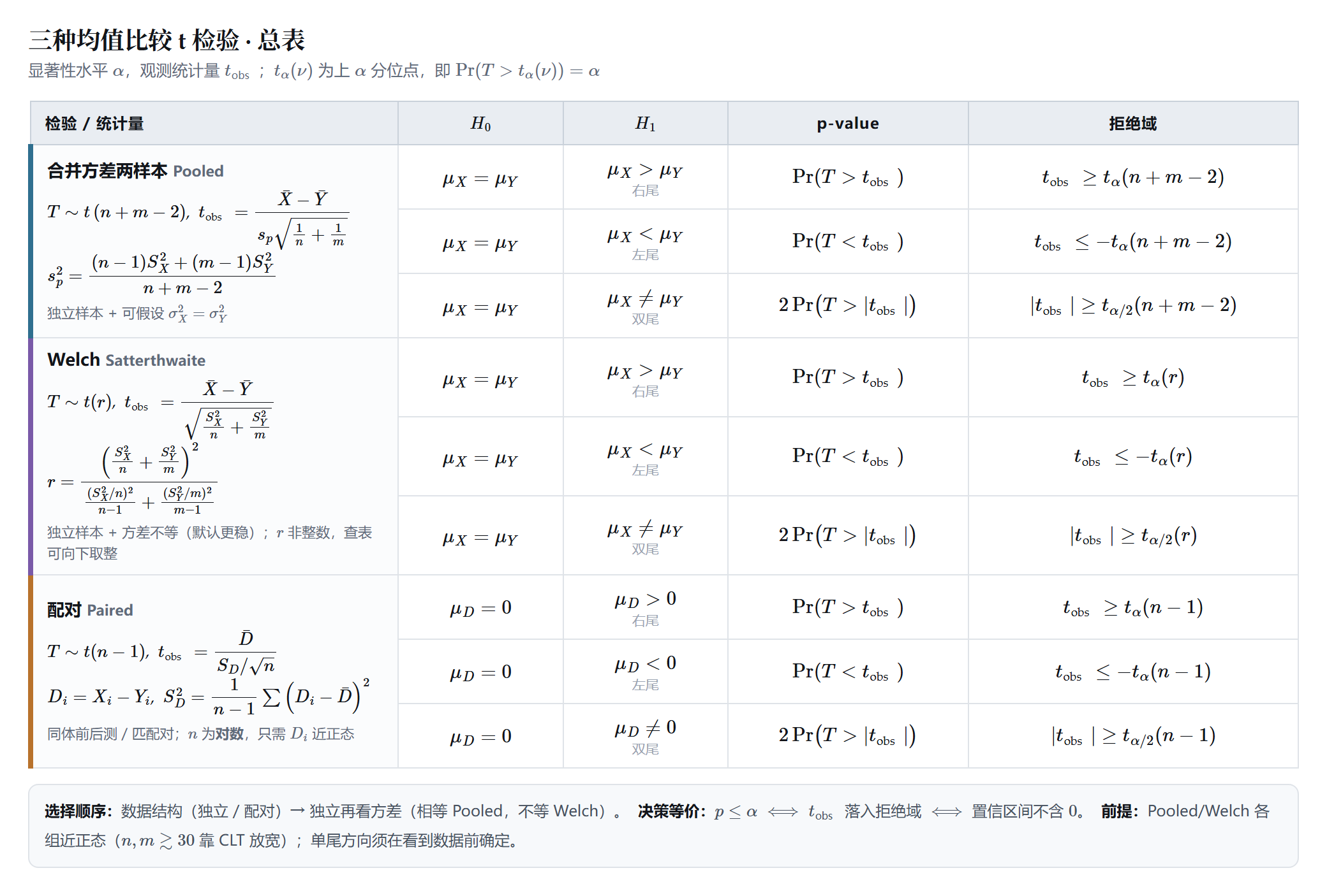
Test versus 3 cases:
Pooled -test
and are independent
are unknown
Welch's -test
and are independent
are unknown
Paired -test
and are independent pairs
Pooled -test
Consider the pooled -test statistic
The pooled variance is
Under ,
Once data and is observed, we can compute
For one-sided test versus -value is
Decision rules: Reject at significance level when either
OR
OR
For one-sided test versus -value is
Decision rules: Reject at significance level when either
OR
OR
For two-sided test versus -value is
Decision rules: Reject at significance level when either
Decision rules: Reject at significance level when either
OR
OR
Note
Same as previous interval,
It is just the paired -interval
Example
24 girls in the 9th and 10th grades were put on an ultraheavy rope-jumping program. Someone thought that such a program would increase their speed in the 40-yard dash. Let equal the difference in time to run the 40-yard dash-the "before-program time" () minus the "after-program time" (). Assume that the distribution of is approximately . We shall test against at significance level . We observe , , .
Test Equality of Two Normal Variances
Suppose two independent populations with i.i.d. samples
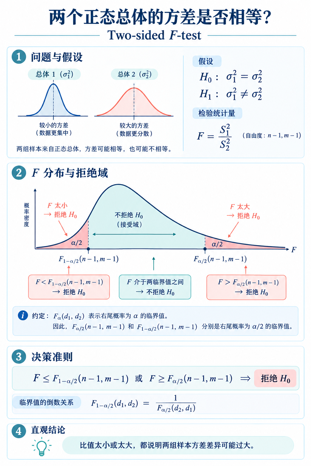
To test versus , we have
Recall -distribution definition,
F-distribution
If independent, then
Define test statistic
Under , the ratio becomes
Once data and is observed, we can compute
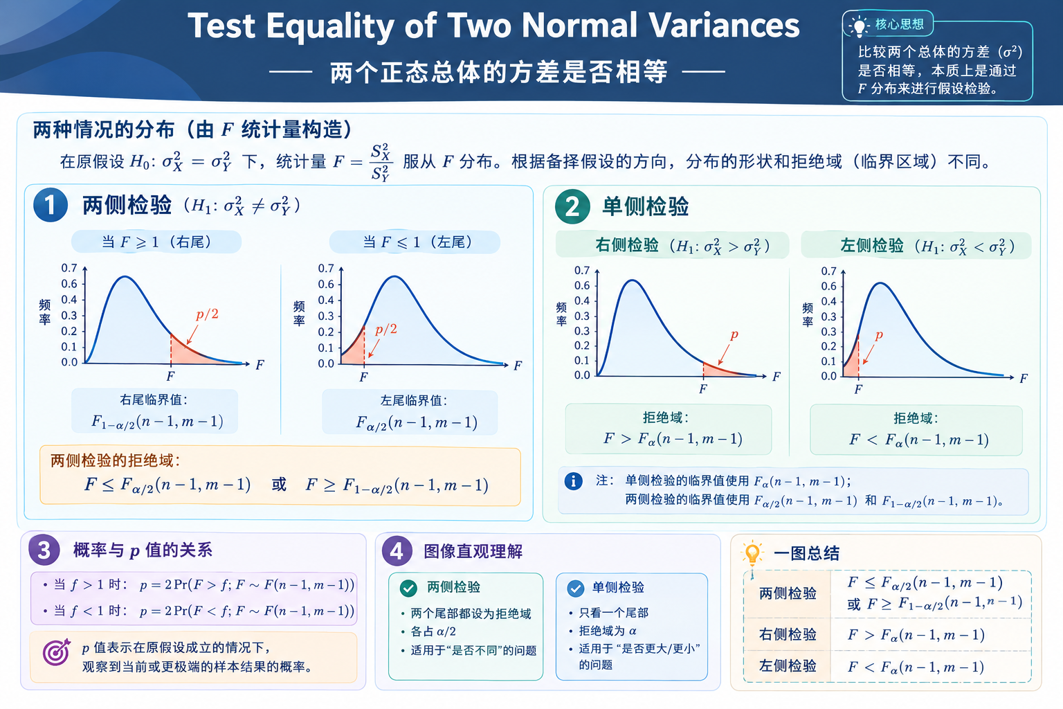
Reject at significance level when
Note
For distribution,
For two-sided test versus
When , -value is
When , -value is
Note
,
左边的 :是一个随机变量,就是 。代入数据后得到观测值 ,它是一个数。
右边的 :是 F 分布(F-distribution)。
Decision rules: Reject at significance level when either
OR
数据关系
方差假设
统计量分母
自由度
何时用它
Pooled
独立
独立且方差相等
Welch
独立
(修正)
独立且方差不等
Paired
配对
只看差值
同一批人测两次
Hypothesis Testing for Proportions
Let be the proportion of population who has certain characteristic To estimate , draw i.i.d. random samples
where each is when it has the characteristic and if doesn't have
Denote , then
If is large enough, by CLT,
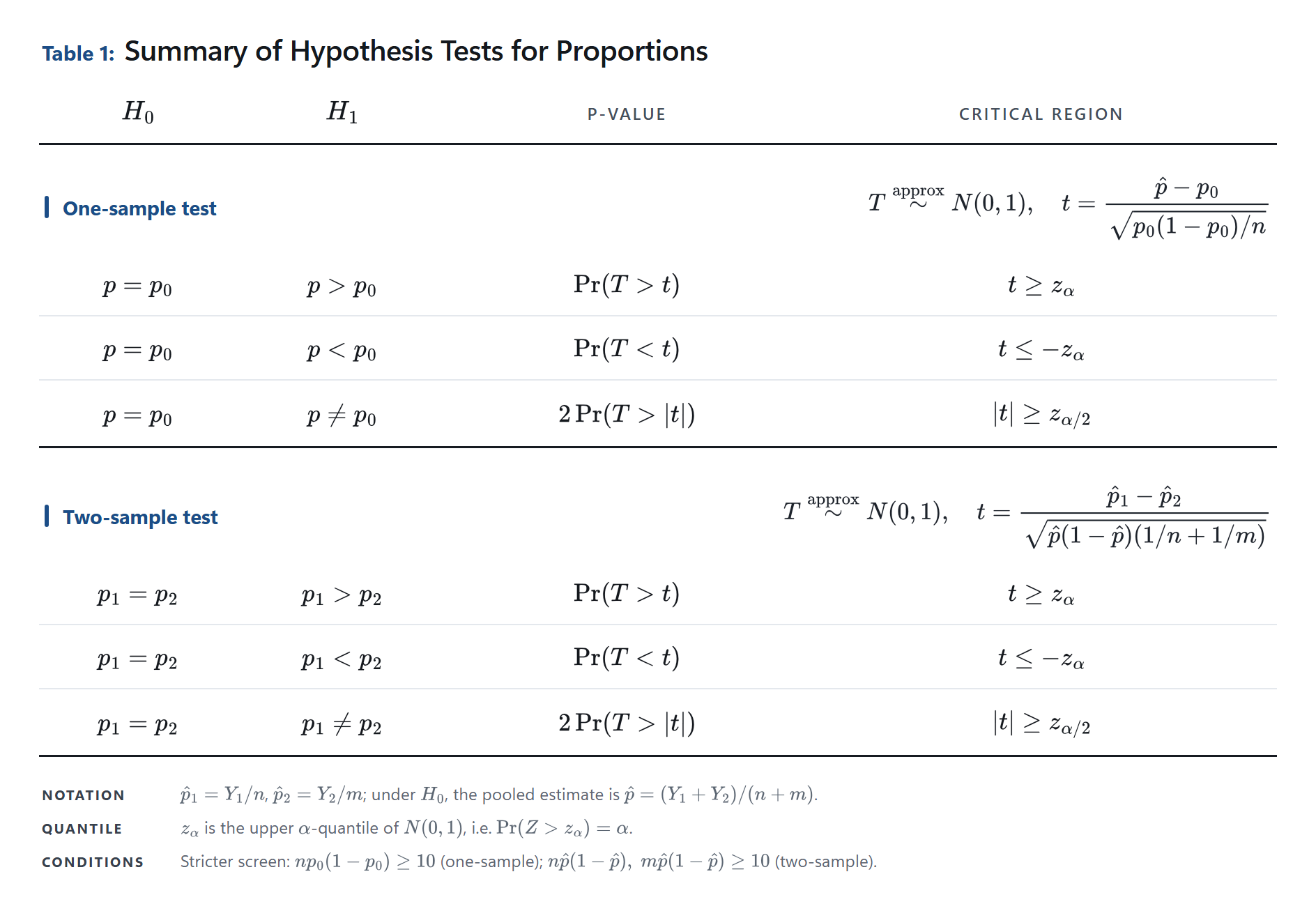
Given null hypothesis test , construct test statistic as follow
Under , approximately
Once data , are observed, we can compute
is the realized value of (即 是 的观测值)
For one-sided test: -value is
where
Reject at significance level when either
-value OR
OR
For one-sided test: -value is
Reject at significance level when either
-value OR
OR
For two-sided test -value is
Reject at significance level when either
-value OR
OR
or
Example
It was claimed that many commercially manufactured dice are not fair because the “spots” are really indentations, so that, for example, the 6-side is lighter than the 1-side. Let equal the probability of rolling a 6 with one of these dice. To test against the alternative hypothesis with significance level , several such dice will be rolled to yield a total of observations, and the number 6 appears 1389 times.
Let be the no. of times that 6 resulted in the 8000 trials. Then, the test statistics is
Critical region approach:
Hence, fail to reject at significance level
-value approach
- Hence, fail to reject at significance level If set with , will be rejected at significance level
这就是为什么统计上严禁“先看 p 值,再挑一个刚好能拒绝 的 ”(这是 p-hacking,也就是操纵数据/分析方式)。 必须在看数据之前定死。而且报告时正确说法是“在 10% 显著性水平下拒绝”,而不是“骰子确实不公平”。
Hypothesis Testing for Equality of Two Proportions
Given there are 2 populations, namely population 1 and population 2. Let and be the proportion of population 1 and 2 respectively, who has a certain characteristic.
Test on against possible alternative hypothesis
Denote the samples to be
Assume they're independent
Denote the sums to be
MLE of are
If are large enough, then by CLT,
For two-sided test Under , and
Approximate by
Construct test statistic
Under ,
Once data are observed, we can compute
-value is
Reject at significance level when either
-value OR
OR
Example
In a sample of , we have low birth weight babies in Country 1. In a sample of we find low birth weight babies in Country 2 Please test versus at significance level