Parameter Estimation

Data Visualization

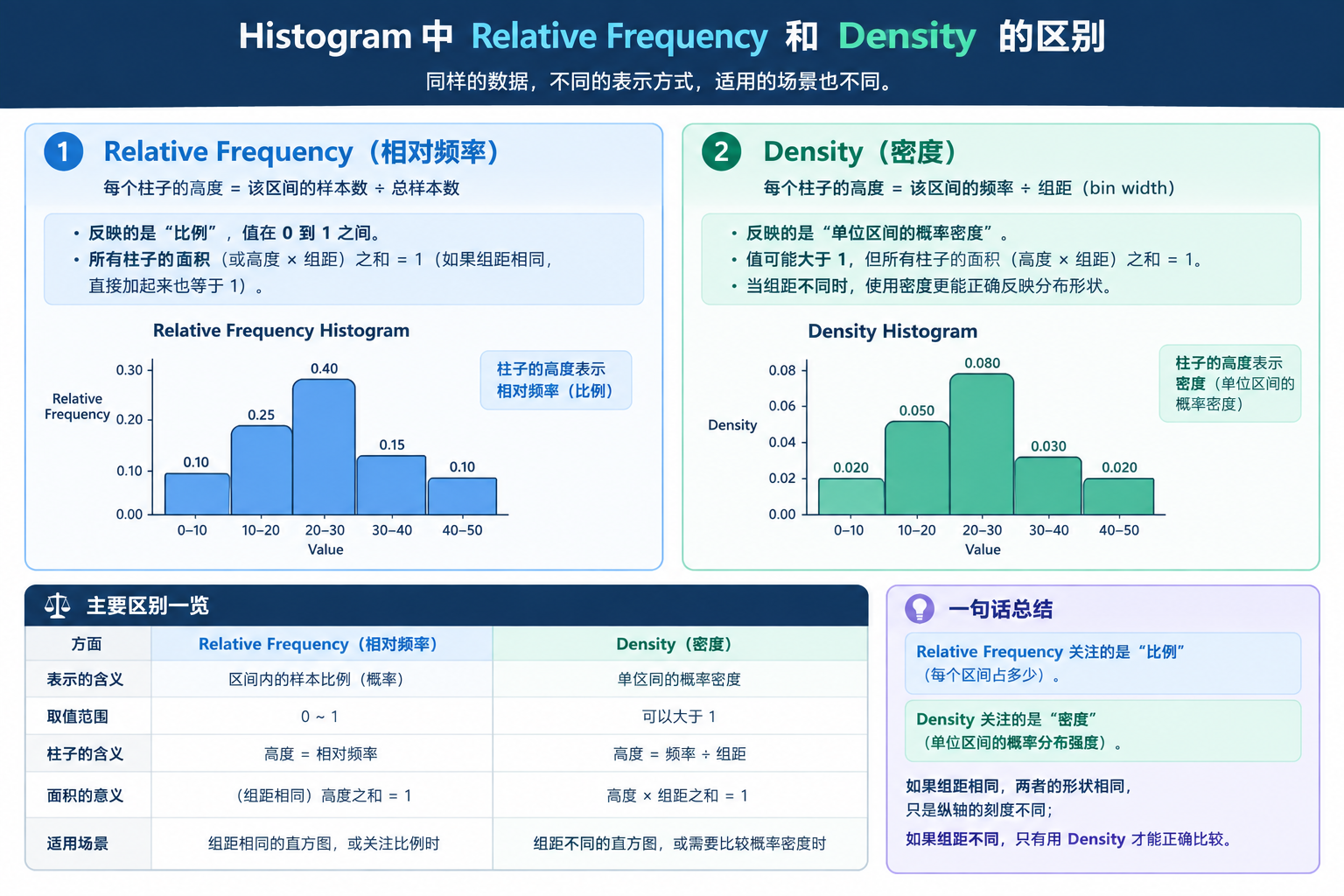
Histogram is used to visualize continuous observations by grouping data into several bins

Height: Relative frequency / density of data points
- Relative frequency: $\frac{# of data in the bin}{# of total data}$
- Density: $\frac{Relative frequency}{Bin width}$
- Let there are $k$ bins, the bin width of $j$ be $w_{j}$ , and the number of data observed in the bin is $n_{j}$ .
  - Relative frequency = $\frac{n_{j}}{n}$
  - Density = $\frac{n_{j}}{w_{j} n}$
    - Sum of areas of all bins always equal to 1: $\sum_{j = 1}^{k} w_{j} (\frac{n_{j}}{w_{j} n}) = 1$
Area: Proportional to the num. of observations
In PDF, probability is the area under the density curve.
Histogram is the discrete version for PDF.

The bin size (num. of bins) is important

Too small: Overfit
Too large: Hide important details & patterns in the data

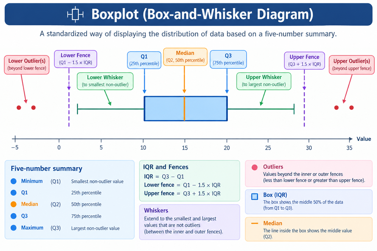
Boxplot

min, \overset{Interquartile range}{\overset{⏞}{\underset{\frac{1}{4}}{\underset{⏟}{Q_{1}}}, \underset{median}{\underset{⏟}{Q_{2}}}, \underset{\frac{3}{4}}{\underset{⏟}{Q_{3}}}}}, max

IQR = $Q_{3} - Q_{1}$
Fence
- Inner fence: Left /right of box at distance $(1.5 \times I Q R)$
- Outer fence: Left / right of box at distance $(3 \times I Q R)$
Whisker
- Lower whisker: From $Q_{1}$ down to the smallest observation $\geq Q_{1} - 1.5 \times I Q R$
- Upper whisker: From $Q_{3}$ up to the largest observation $\leq Q_{3} + 1.5 \times I Q R$
Suspect outlier: Between inner & outer fence $(Q_{3} + 3 \times I Q R > x > Q_{3} + 1.5 \times I Q R)$ or $(Q_{1} - 3 \times I Q R < x < Q_{1} - 1.5 \times I Q R)$
Outlier: Beyond the outer fence ( $x > Q_{3} + 3 \times I Q R$ or $x < Q_{1} - 3 \times I Q R$ )

Interpretation

Box shows the middle 50% of data
Whiskers show the range of normal data points
- i.e. data within $\pm 1.5 \times I Q R$ are normal
- Left-skewed: Lower whisker is longer than upper whisker
- Right-skewed: Upper whisker is longer than lower whisker
Data beyond outer fence are outliers
Boxplot shows the variance & skewness of data + identify outliers

Parameter Estimation / Point Estimation

Given a sample with size $n$ from population
Assumption:

Sample is representative of the population
Data are i.i.d.

Parameter Space

Suppose sample $X_{1}, \dots, X_{n}$ are random and i.i.d. with unknown parameter $θ$ and PMF / PDF $f (x; θ)$ .
The parameter $θ$ takes value in the parameter space $Ω$ (i.e. domain of $θ$ )

Note

在之后求解 MLE 时起到硬约束的作用（不可以取超过 $Ω$ 的值）

Example
For the PDF of normal distribution,
$f (x) = \frac{1}{σ \sqrt{2 π}} \exp [- \frac{(x - μ)^{2}}{2 σ^{2}}], - \infty < x < \infty$

Hence, the corresponding parameter space is
$Ω = {(μ, σ^{2}) : - \infty < μ < \infty, 0 < σ^{2} < \infty}$

$μ$ 可以取任意 real number
$σ^{2}$ 必然是 positive number，必然大于 0

Estimator

写法	名称	性质	例子
大写 $X_{i}$	随机变量（random variable）	在抽样之前，结果是未知的，是随机的	"下一位被测者的身高"
小写 $x_{i}$	观测值（observed value）	抽样之后，已经拿到手的确定数值	我实际测到 172.5 cm

Estimator of $θ$ : $\hat{θ} = u (X_{1}, X_{2}, \dots, X_{n})$
Estimate of $θ$ : Value of $u (x_{1}, x_{2}, \dots, x_{n})$
Since $u (X_{1}, X_{2}, \dots, X_{n})$ outputs a single value, it is called a point estimator

\underset{Point estimator：Random variables}{\underset{⏟}{u (X_{1}, \dots, X_{n})}} \overset{代入具体样本}{\to} \underset{point estimate：Single value}{\underset{⏟}{u (x_{1}, \dots, x_{n})}} \overset{用来猜}{\to} \underset{真参数：永远不知道}{\underset{⏟}{θ}}

Evaluate estimate

偏差 Bias: $Bias (\hat{θ}) = E (\hat{θ}) - θ$
Variance: $Var (\hat{θ}) = E [{(\hat{θ} - E \hat{θ})}^{2}]$
Mean square error (MSE): $\underset{总误差 MSE}{\underset{⏟}{E [(\hat{θ} - θ)^{2}]}} = \underset{抖（精度）}{\underset{⏟}{Var (\hat{θ})}} + \underset{偏（准确度）}{\underset{⏟}{{[E (\hat{θ}) - θ]}^{2}}}$
Consistency: $lim_{n \to \infty} Pr (| \hat{θ} - θ | > ε) = 0$
- 评估样本多了会不会变好

Maximum Likelihood Estimation

Estimator

\begin{aligned} L (θ) & := f (x_{1}, x_{2}, \dots, x_{n}; θ) = \prod_{i = 1}^{n} f (x_{i}; θ) \\ ℓ (θ) & := \ln L (θ) \end{aligned}

$L (θ) \to ℓ (θ)$ 使得乘积变成求和，方便求导计算

Maximum likelihood estimator (MLE) $\hat{θ}$ : Value of $θ$ that maximizes $L (θ)$

\hat{θ} = \arg max_{θ \in Ω} L (θ)

Calculation of MLE

Formulate $ℓ (θ)$
$\underset{score function}{\underset{⏟}{\frac{\partial ℓ (θ)}{\partial θ}}} = 0 \Rightarrow \hat{θ}$
1. 这一步的 $\hat{θ}$ 只是 stationary point，不一定是 maximum point
$- {\frac{\partial^{2} ℓ (θ)}{\partial θ^{2}} |}_{θ = \hat{θ}} > 0 \Rightarrow \hat{θ} is MLE$

Example

Bernoulli Distribution

Formulate $ℓ (θ)$

\begin{aligned} f (x; p) & = p^{x} (1 - p)^{1 - x}, x \in {0, 1}, 0 \leq p \leq 1 \\ L (p) & = \prod_{i = 1}^{n} p^{x_{i}} (1 - p)^{1 - x_{i}} \\ = p^{\sum_{i = 1}^{n} x_{i}} (1 - p)^{\sum_{i = 1}^{n} 1 - x_{i}} \\ = p^{\sum_{i = 1}^{n} x_{i}} (1 - p)^{n - \sum_{i = 1}^{n} x_{i}} \\ ℓ (p) & = (\sum_{i = 1}^{n} x_{i}) \ln p + (n - \sum_{i = 1}^{n} x_{i}) \ln (1 - p) \end{aligned}

Use score function to find MLE

\begin{aligned} ℓ^{'} (p) & = 0 \\ (\sum_{i = 1}^{n} x_{i}) \frac{1}{p} - (n - \sum_{i = 1}^{n} x_{i}) \frac{1}{1 - p} & = 0 \\ (\sum_{i = 1}^{n} x_{i}) \frac{1}{p} & = (n - \sum_{i = 1}^{n} x_{i}) \frac{1}{1 - p} \\ (1 - p) (\sum_{i = 1}^{n} x_{i}) & = p (n - \sum_{i = 1}^{n} x_{i}) \\ \sum_{i = 1}^{n} x_{i} - p \sum_{i = 1}^{n} x_{i} & = p n - p \sum_{i = 1}^{n} x_{i} \\ \sum_{i = 1}^{n} x_{i} & = p n \\ p & = \frac{1}{n} \sum_{i = 1}^{n} x_{i} \\ \hat{p} & = \bar{x} \end{aligned}

Verify $\hat{θ}$ is MLE

\begin{aligned} ℓ^{″} (p) & = - \frac{\sum_{i = 1}^{n} x_{i}}{p^{2}} - (n - \sum_{i = 1}^{n} x_{i}) \frac{1}{(1 - p)^{2}} \\ ∵ \sum_{i = 1}^{n} x_{i} \geq 0 & , n - \sum_{i = 1}^{n} x_{i} \geq 0 \\ ℓ^{″} (p) & < 0 \end{aligned}

Since $ℓ^{″} (p) < 0$ , $ℓ (p)$ is strictly concave function, $\hat{p} = \bar{x}$ is the MLE.
The MLE is the sample mean in Bernoulli Distribution.

Exponential Distribution

\begin{aligned} f (x; θ) & = \frac{1}{θ} e^{- x / θ}, 0 < x < \infty, θ \in (0, \infty) \\ L (θ) & = \frac{1}{θ^{n}} \exp (- \frac{\sum_{i = 1}^{n} x_{i}}{θ}) \\ ℓ (θ) & = - \frac{\sum_{i = 1}^{n} x_{i}}{θ} + \ln \frac{1}{θ^{n}} \\ = - \frac{\sum_{i = 1}^{n} x_{i}}{θ} - n \ln θ \\ ℓ^{'} (θ) & = 0 \\ \frac{\sum_{i = 1}^{n} x_{i}}{θ^{2}} - \frac{n}{θ} & = 0 \\ \frac{\sum_{i = 1}^{n} x_{i}}{θ^{2}} & = \frac{n}{θ} \\ θ & = \frac{1}{n} \sum_{i = 1}^{n} x_{i} \\ \hat{θ} & = \bar{x} \\ ℓ^{″} (θ) & = - \frac{2 \sum_{i = 1}^{n} x_{i}}{θ^{3}} + \frac{n}{θ^{2}} \\ = - \underset{\bar{x} = \frac{1}{n} \sum_{i = 1}^{n} x_{i}}{\underset{⏟}{\frac{2 n \bar{x}}{θ^{3}}}} + \frac{n}{θ^{2}} \\ ℓ^{″} (θ) |_{θ = \bar{x}} & = - \frac{2 n \bar{x}}{{\bar{x}}^{3}} + \frac{n}{{\bar{x}}^{2}} \\ = - \frac{2 n}{{\bar{x}}^{2}} + \frac{n}{{\bar{x}}^{2}} \\ = - \frac{n}{{\bar{x}}^{2}} \\ < 0 \end{aligned}

Hence, $\hat{θ} = \bar{x}$ is the MLE for Exponential Distribution.

Poisson Distribution

\begin{aligned} f (x; λ) & = \frac{λ^{x}}{x!} e^{- λ} \\ L (λ) & = \prod_{i = 1}^{n} \frac{λ^{x_{i}}}{x_{i}!} e^{- λ} \\ = \frac{λ^{\sum_{i = 1}^{n} x_{i}}}{\prod_{i = 1}^{n} x_{i}!} e^{- n λ} \\ ℓ (λ) & = \sum_{i = 1}^{n} x_{i} \ln λ - \ln (\prod_{i = 1}^{n} x_{i}!) - n λ \\ ℓ^{'} (λ) & = \frac{1}{λ} \sum_{i = 1}^{n} x_{i} - n \\ 0 & = \frac{n \bar{x}}{λ} - n \\ n λ & = n \bar{x} \\ \hat{λ} & = \bar{x} \\ - ℓ^{″} (λ) & = \frac{1}{λ^{2}} \sum_{i = 1}^{n} x_{i} \\ - ℓ^{″} (λ) |_{λ = \bar{x}} & = \frac{1}{{\bar{x}}^{2}} \sum_{i = 1}^{n} x_{i} \\ = \frac{1}{{\bar{x}}^{2}} n \bar{x} \\ = \frac{n}{\bar{x}} \\ > 0 \end{aligned}

Geometric Distribution

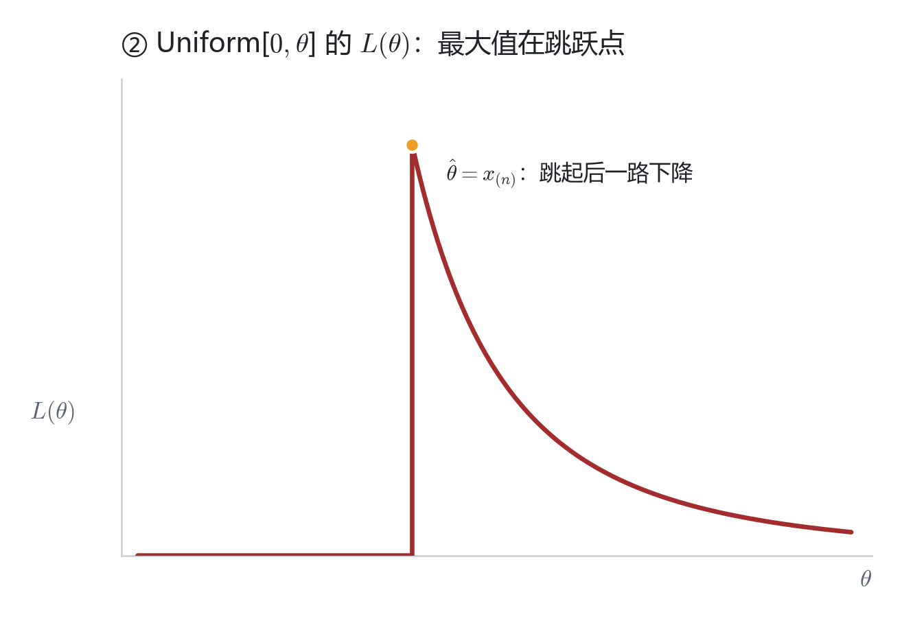
\begin{aligned} f (x; p) & = (1 - p)^{x - 1} p \\ L (p) & = \prod_{i = 1}^{n} (1 - p)^{x_{i} - 1} p \\ = (1 - p)^{\sum_{i = 1}^{n} x_{i} - n} p^{n} \\ ℓ (p) & = (\sum_{i = 1}^{n} x_{i} - n) \ln (1 - p) + n \ln p \\ ℓ^{'} (p) & = 0 \\ 0 & = - \frac{1}{1 - p} (\sum_{i = 1}^{n} x_{i} - n) + \frac{n}{p} \\ \frac{n \bar{x} - n}{1 - p} & = \frac{n}{p} \\ \frac{\bar{x} - 1}{1 - p} & = \frac{1}{p} \\ p (\bar{x} - 1) & = 1 - p \\ p \bar{x} & = 1 \\ \hat{p} & = \frac{1}{\bar{x}} \\ - ℓ^{″} (p) & = \frac{1}{(1 - p)^{2}} (\sum_{i = 1}^{n} x_{i} - n) + \frac{n}{p^{2}} \\ = \frac{1}{(1 - p)^{2}} (n \bar{x} - n) + \frac{n}{p^{2}} \\ - ℓ^{″} (p) |_{p = \frac{1}{\bar{x}}} & = \frac{1}{{(1 - \frac{1}{\bar{x}})}^{2}} (n \bar{x} - n) + \frac{n}{\frac{1}{{\bar{x}}^{2}}} \\ = \frac{{\bar{x}}^{2} (n \bar{x} - n)}{(\bar{x} - 1)^{2}} + {\bar{x}}^{2} n \\ = \frac{n {\bar{x}}^{2} (\bar{x} - 1)}{(\bar{x} - 1)^{2}} + {\bar{x}}^{2} n \\ = n {\bar{x}}^{2} [\frac{\bar{x} - 1}{(\bar{x} - 1)^{2}} + 1] \\ > 0 \end{aligned}

Uniform Distribution (Special Cases)

\begin{aligned} f (x) & = {\begin{cases} \frac{1}{θ}, 0 \leq x \leq θ, \\ 0, Otherwise \end{cases} θ \in (0, \infty) \end{aligned}

For the likelihood function $L (θ)$ ,

L (θ) = \prod_{i = 1}^{n} f (x_{i}; θ)

If $x_{i} > θ$ or $x_{i} < 0$ , then $f (x_{i}) = 0$ and $L (θ) = 0$
Hence, $L (θ) > 0 ⟺$

$0 \leq min_{i} x_{i}$ and
$max {x_{1}, x_{2}, \dots, x_{n}} \leq θ$

L (θ) = {\begin{cases} \frac{1}{θ^{n}}, & θ \geq max_{i} x_{i} \\ 0, & θ < max_{i} x_{i} \end{cases}

However, we cannot use $ℓ^{'} (θ) = 0$ to find $\hat{θ}$ because $\hat{θ}$ is on the boundary or at a discontinuous point.

Hence, we need to introduce indicator function to rewrite $L (θ)$ .
Indicator function is

1 {A} = {\begin{cases} 1, & 若条件 A 成立 \\ 0, & 若条件 A 不成立 \end{cases}

Rewrite $L (θ)$ ,

\begin{aligned} f (x; θ) & = \frac{1}{θ} 1_{{x \in [0, θ]}} \\ L (θ) & = \prod_{i = 1}^{n} \frac{1}{θ} 1_{{x \in [0, θ]}} \\ = \frac{1}{θ^{n}} 1_{{0 \leq min_{i} {x_{i}}, max_{i} {x_{i}} \leq θ}} \\ = {\begin{cases} θ^{- n}, & θ \geq max_{i} x_{i} \\ 0, & Otherwises \end{cases} \end{aligned}

The domain of $L (θ)$ now becomes $θ \in [max_{i} x_{i}, \infty)$ .
Hence, $\hat{θ} = max_{i} {x_{i}}$ , which is the min. point within the domain.

Definition

Maximum Likelihood Estimator
$\hat{θ} = \hat{θ} (X_{1}, \dots, X_{n})$ is MLE of $θ$ if

\hat{θ} = \arg max L (θ; X_{1}, \dots, X_{n})

It means $L (θ; X_{1}, \dots, X_{n})$ achieves its max. value at $\hat{θ}$

Unbiased Estimator

Definition

An estimator $u (X_{1}, X_{2}, \dots, X_{n})$ of $θ$ is unbiased estimator of $θ$ if

E [u (X_{1}, X_{2}, \dots, X_{n})] = θ

Otherwise, $u (X_{1}, X_{2}, \dots, X_{n})$ is biased estimator

Example

Calculate the MLE of normal distribution.

\begin{aligned} X_{1}, \dots, X_{n} & \sim N (\underset{μ}{\underset{⏟}{θ_{1}}}, \underset{σ^{2}}{\underset{⏟}{θ_{2}}}) \\ f (x; θ) & = \frac{1}{\sqrt{2 π θ_{2}}} \exp [- \frac{(x - θ_{1})^{2}}{2 θ_{2}}], - \infty < x < \infty \\ θ \in Ω & = {(θ_{1}, θ_{2}) : - \infty < θ_{1} < \infty ， 0 < θ_{2} < \infty} \\ L (θ_{1}, θ_{2}) & = \prod_{i = 1}^{n} \frac{1}{\sqrt{2 π θ_{2}}} \exp [- \frac{(x - θ_{1})^{2}}{2 θ_{2}}] \\ = \frac{1}{{(\sqrt{2 π θ_{2}})}^{n}} \exp [- \frac{\sum_{i = 1}^{n} (x_{i} - θ_{1})^{2}}{2 θ_{2}}] \\ ℓ (θ_{1}, θ_{2}) & = - \frac{n}{2} \ln (2 π θ_{2}) - \frac{\sum_{i = 1}^{n} (x_{i} - θ_{1})^{2}}{2 θ_{2}} \\ = - \frac{n}{2} \ln (2 π) - \frac{n}{2} \ln θ_{2} - \frac{\sum_{i = 1}^{n} (x_{i} - θ_{1})^{2}}{2 θ_{2}} \\ \frac{\partial ℓ (θ_{1}, θ_{2})}{\partial θ_{1}} & = \frac{\sum_{i = 1}^{n} (x_{i} - θ_{1})}{θ_{2}} \\ 0 & = \frac{\sum_{i = 1}^{n} (x_{i} - θ_{1})}{θ_{2}} \\ \sum_{i = 1}^{n} (x_{i} - θ_{1}) & = 0 \\ \sum_{i = 1}^{n} x_{i} - n θ_{1} & = 0 \\ θ_{1} & = \frac{1}{n} \sum_{i = 1}^{n} x_{i} \\ {\hat{θ}}_{1} & = \bar{x} \\ \frac{\partial ℓ (θ_{1}, θ_{2})}{\partial θ_{2}} & = \frac{\sum_{i = 1}^{n} (x_{i} - θ_{1})^{2}}{2 θ_{2}^{2}} - \frac{n}{2 θ_{2}} \\ 0 & = \frac{\sum_{i = 1}^{n} (x_{i} - θ_{1})^{2}}{2 θ_{2}^{2}} - \frac{n}{2 θ_{2}} \\ n θ_{2} & = \sum_{i = 1}^{n} (x_{i} - θ_{1})^{2} \\ {\hat{θ}}_{2} & = \frac{1}{n} \sum_{i = 1}^{n} (x_{i} - θ_{1})^{2} \\ {\begin{cases} {\hat{θ}}_{1} & = \bar{x} \\ {\hat{θ}}_{2} & = \frac{1}{n} \sum_{i = 1}^{n} (x_{i} - θ_{1})^{2} \end{cases} \\ - \frac{\partial^{2} ℓ (θ_{1}, θ_{2})}{\partial θ_{1} \partial θ_{2}} & = - [\begin{array}{c} \frac{\partial^{2} ℓ (θ_{1}, θ_{2})}{\partial θ_{1}^{2}} & \frac{\partial^{2} ℓ (θ_{1}, θ_{2})}{\partial θ_{2} \partial θ_{1}} \\ \frac{\partial^{2} ℓ (θ_{1}, θ_{2})}{\partial θ_{1} \partial θ_{2}} & \frac{\partial^{2} ℓ (θ_{1}, θ_{2})}{\partial θ_{2}^{2}} \end{array}] \\ {\begin{cases} - \frac{\partial^{2} ℓ (θ_{1}, θ_{2})}{\partial θ_{1}^{2}} & = \frac{n}{θ_{2}} \\ - \frac{\partial^{2} ℓ (θ_{1}, θ_{2})}{\partial θ_{2} \partial θ_{1}} & = \frac{\sum_{i = 1}^{n} x_{i}}{θ_{2}^{2}} - \frac{n θ_{1}}{θ_{2}^{2}} = \frac{n (\bar{x} - θ_{1})}{θ_{2}^{2}} \\ \frac{\partial^{2} ℓ (θ_{1}, θ_{2})}{\partial θ_{2}^{2}} & = - \frac{n}{2 θ_{2}^{2}} + \frac{\sum_{i = 1}^{n} (x_{i} - θ_{1})^{2}}{2 θ_{2}^{3}} \end{cases} \\ - \frac{\partial^{2} ℓ (θ_{1}, θ_{2})}{\partial θ_{1} \partial θ_{2}} & > 0 \\ ∴ & {\begin{cases} {\hat{θ}}_{1} & = \bar{x} \\ {\hat{θ}}_{2} & = \frac{1}{n} \sum_{i = 1}^{n} (x_{i} - θ_{1})^{2} \end{cases} \end{aligned}

Given that sample variance $S^{2} = \frac{1}{n - 1} \sum_{i = 1}^{n} (X_{i} - \bar{X})^{2}$
Rewrite ${\hat{θ}}_{2}$ as

\begin{aligned} {\hat{θ}}_{2} & = \frac{1}{n} \sum_{i = 1}^{n} (x_{i} - θ_{1})^{2} \\ = \frac{n - 1}{n} [\frac{1}{n - 1} \sum_{i = 1}^{n} (X_{i} - \bar{X})^{2}] \\ = \frac{n - 1}{n} S^{2} \end{aligned}

Recall that

\begin{aligned} \bar{X} & \sim N (θ_{1}, \frac{θ_{2}}{n}) \\ \frac{(n - 1) S^{2}}{θ_{2}} & \sim χ^{2} (n - 1) \end{aligned}

Hence,

\begin{aligned} E ({\hat{θ}}_{1}) & = E (\bar{X}) \\ = μ \\ = θ_{1} \\ E (S^{2}) & = E {(\frac{θ_{2}}{n - 1}) [\frac{(n - 1) S^{2}}{θ_{2}}]} \\ = \frac{θ_{2}}{n - 1} E [\frac{(n - 1) S^{2}}{θ_{2}}] \\ = \frac{θ_{2}}{n - 1} E [χ^{2} (n - 1)] \\ = \frac{θ_{2}}{n - 1} (n - 1) \\ = θ_{2} \\ E (\hat{θ_{2}}) & = \frac{n - 1}{n} E (S^{2}) \\ = \frac{n - 1}{n} θ_{2} \end{aligned}

Hence, ${\hat{θ}}_{1}$ is unbiased estimator while ${\hat{θ}}_{2}$ is biased estimator of $θ_{2}$

Method of Moments (MoM)

As MLE may not able to find an explicit formula for the max. value, it requires numerical optimization.

For the unknown parameter $θ = (θ_{1}, \dots, θ_{n})$ is $k$ -dimensional.
For $1 \leq j \leq k$ , denote the $j^{t h}$ moment to be

α_{j} (θ) = E_{θ} (X^{j})

Denote the $j^{t h}$ sample moment to be

{\hat{α}}_{j} = \frac{1}{n} \sum_{i = 1}^{n} X_{i}^{j}

Definition

Method of Moments Estimator
The method of moments estimator $\hat{θ}$ is defined to be the value of $θ$ s.t.

\begin{aligned} α_{1} (θ) & = {\hat{α}}_{1} \\ α_{2} (θ) & = {\hat{α}}_{2} \\ ⋮ \\ α_{k} (θ) & = {\hat{α}}_{k} \end{aligned}

It gives a system of $k$ equations with $k$ unkwown

Note

为什么“矩”可以估计参数？
因为不同参数会让分布的理论平均值不同；观察到样本平均值后，就可以反推参数

如果 $λ = 1$ ，Poisson 数据通常集中在 0、1、2。
如果 $λ = 10$ ，Poisson 数据通常会在 10 附近。
如果样本均值是 1.6，我们自然会觉得 $λ$ 大概在 1.6 附近。
MoM 就是把这个直觉数学化：

理论平均 = 样本平均

Example

Gamma Distribution

For $X_{1}, \dots, X_{n} \sim Gamma (θ_{1}, θ_{2})$ . The unknown parameter is two-dimensional $θ = (θ_{1}, θ_{2})$ .
The first two moments are

\begin{aligned} α_{1} (θ_{1}, θ_{2}) & = E_{θ} (X_{1}) = θ_{1} θ_{2} \\ α_{2} (θ_{1}, θ_{2}) & = E_{θ} (X_{1}^{2}) = θ_{1} θ_{2} + θ_{1}^{2} θ_{2}^{2} \end{aligned}

The first two sample moments are

\begin{aligned} {\hat{α}}_{1} & = \frac{1}{n} \sum_{i = 1}^{n} X_{i} \\ {\hat{α}}_{2} & = \frac{1}{n} \sum_{i = 1}^{n} X_{i}^{2} \end{aligned}

The $k^{t h}$ moment $α_{k} (θ)$ is equal to $k^{t h}$ sample moment ${\hat{α}}_{k}$

{\begin{cases} θ_{1} θ_{2} & = \frac{1}{n} \sum_{i = 1}^{n} X_{i} = \bar{X} \\ θ_{1} θ_{2}^{2} + θ_{1}^{2} θ_{2}^{2} & = \frac{1}{n} \sum_{i = 1}^{n} X_{i}^{2} \end{cases}

\begin{aligned} Let V & = \frac{1}{n} \sum_{i = 1}^{n} (X_{i} - \bar{X})^{2} \\ = \frac{1}{n} \sum_{i = 1}^{n} (X_{i}^{2} - 2 \bar{X} X_{i} + {\bar{X}}^{2}) \\ = \frac{1}{n} [\sum_{i = 1}^{n} (X_{i}^{2}) - 2 \sum_{i = 1}^{n} \bar{X} X_{i} + n {\bar{X}}^{2}] \\ = \frac{1}{n} \sum_{i = 1}^{n} (X_{i}^{2}) - 2 {\bar{X}}^{2} + {\bar{X}}^{2} \\ = \frac{1}{n} \sum_{i = 1}^{n} X_{i}^{2} - {\bar{X}}^{2} \end{aligned}

Sub. $θ_{1} θ_{2}$ into $θ_{1} θ_{2}^{2} + θ_{1}^{2} θ_{2}^{2}$ ,

\begin{aligned} \bar{X} θ_{2} + {\bar{X}}^{2} & = \frac{1}{n} \sum_{i = 1}^{n} X_{i}^{2} \\ \bar{X} θ_{2} & = V \\ θ_{2} & = \frac{V}{\bar{X}} \\ θ_{1} θ_{2} & = \bar{X} \\ θ_{1} \frac{V}{\bar{X}} & = \bar{X} \\ θ_{1} & = \frac{{\bar{X}}^{2}}{V} \end{aligned}

Hence, the method of moments estimators are

{\begin{cases} {\tilde{θ}}_{1} & = \frac{{\bar{X}}^{2}}{V} \\ {\tilde{θ}}_{2} & = \frac{V}{\bar{X}} \end{cases}

Poisson Distribution

\begin{aligned} X_{1}, \dots, X_{n} & \sim P (λ) \\ α_{1} (λ) & = E (X) \\ = λ \\ {\hat{α}}_{1} & = \frac{1}{n} \sum_{i = 1}^{n} X_{i} \\ = \bar{X} \\ α_{1} (λ) & = {\hat{α}}_{1} \\ λ & = \bar{X} \\ {\tilde{λ}}_{1} & = \bar{X} \end{aligned}

MoM estimator is not unique for Poisson distribution, i.e. second-moment estimator

\begin{aligned} E (X^{2}) & = E (X^{2}) - [E (X)]^{2} + [E (X)]^{2} \\ = V a r (X) + [E (X)]^{2} \\ = λ + λ^{2} \\ λ & = E (X^{2}) - λ^{2} \\ = E (X^{2}) - [E (X)]^{2} \\ = \frac{1}{n} \sum_{i = 1}^{n} X_{i}^{2} - {\bar{X}}^{2} \\ {\tilde{λ}}_{2} & = \frac{1}{n} \sum_{i = 1}^{n} X_{i}^{2} - {\bar{X}}^{2} \end{aligned}

Note

Mean-based estimator ${\tilde{λ}}_{1} = \bar{X}$ is preferred because of smaller variance.

Uniform Distribution

\begin{aligned} X_{1}, \dots, X_{n} & \sim U (0, θ) \\ α (θ) & = E (X) \\ = \frac{θ}{2} \\ \hat{α} & = \frac{1}{n} \sum_{i = 1}^{n} X_{i} \\ = \bar{X} \\ \frac{θ}{2} & = \bar{X} \\ \tilde{θ} & = 2 \bar{X} \end{aligned}

Note

$\tilde{θ}$ may not be a good estimator if

2 \bar{X} < max {X_{1}, \dots, X_{n}}

As in uniform distribution $U (0, θ)$ , all data are in $(0, θ)$ .
Hence, $θ$ should be larger than $max_{i} {X_{i}}$ .
If $\underset{\tilde{θ}}{\underset{⏟}{2 \bar{X}}} < max {X_{1}, \dots, X_{n}}$ , it is contradiction.